Generate ggplot2 object. — autoplot.smoof

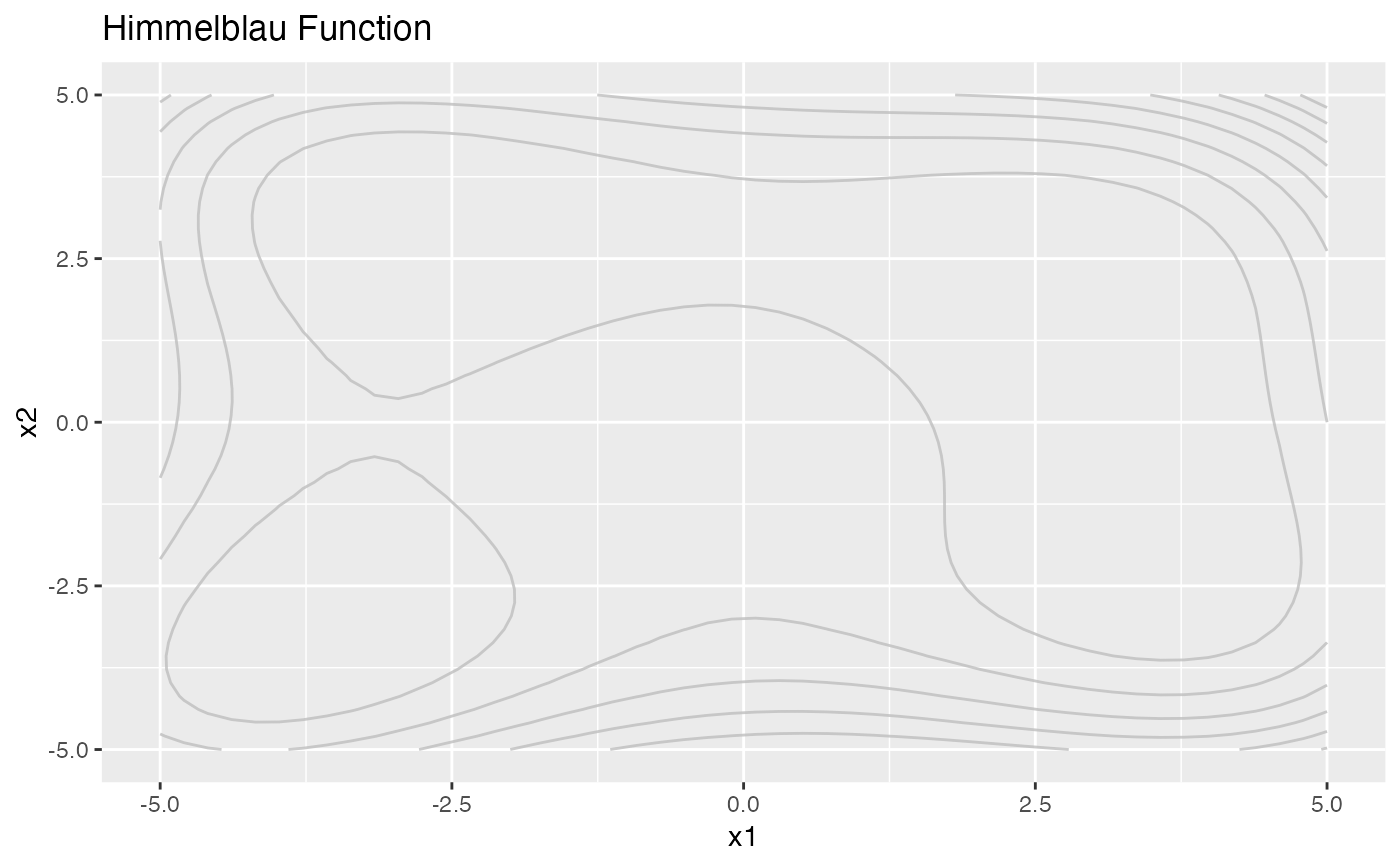
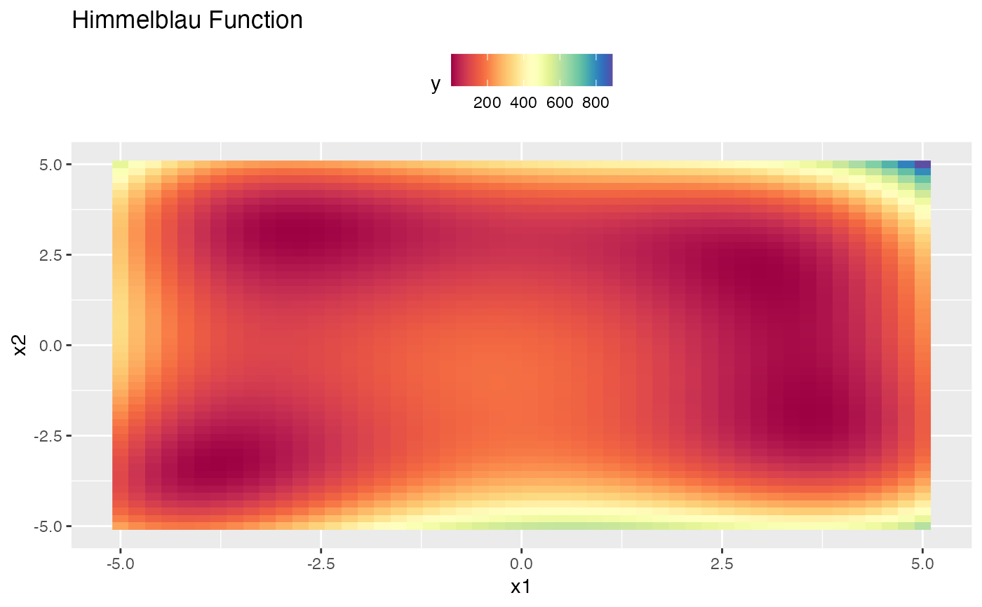
This function expects a smoof function and returns a ggplot object depicting the function landscape. The output depends highly on the decision space of the smoof function or more technically on the ParamSet of the function. The following destinctions regarding the parameter types are made. In case of a single numeric parameter a simple line plot is drawn. 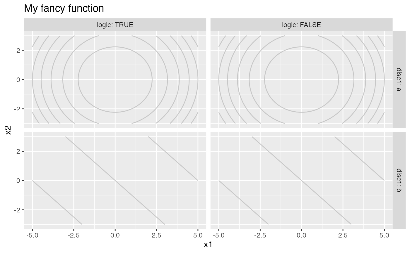For two numeric parameters or a single numeric vector parameter of length 2 either a contour plot or a heatmap (or a combination of both depending on the choice of additional parameters) is depicted. If there are both up to two numeric and at least one discrete vector parameter, ggplot facetting is used to generate subplots of the above-mentioned types for all combinations of discrete parameters.

# S3 method for smoof_function
autoplot(
  object,
  ...,
  show.optimum = FALSE,
  main = getName(x),
  render.levels = FALSE,
  render.contours = TRUE,
  log.scale = FALSE,
  length.out = 50L
)

Arguments

object: [smoof_function]
Objective function.
...: [any]
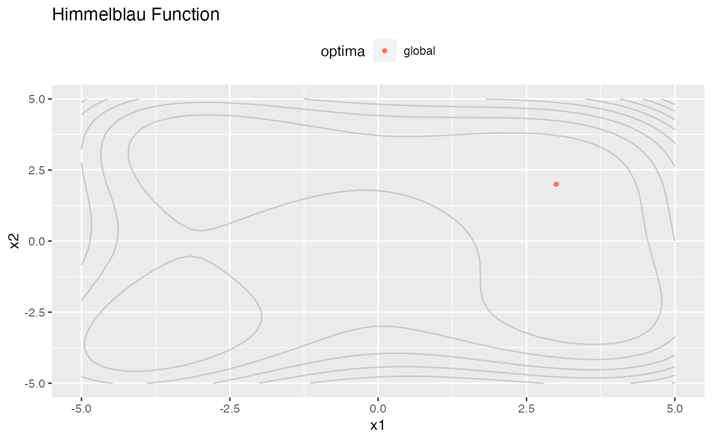
Not used.
show.optimum: [logical(1)]
If the function has a known global optimum, should its location be plotted by a point or multiple points in case of multiple global optima? Default is FALSE.
main: [character(1L)]
Plot title. Default is the name of the smoof function.
render.levels: [logical(1)]
For 2D numeric functions only: Should an image map be plotted? Default is FALSE.
render.contours: [logical(1)]
For 2D numeric functions only: Should contour lines be plotted? Default is TRUE.
log.scale: [logical(1)]
Should the z-axis be plotted on log-scale? Default is FALSE.
length.out: [integer(1)]
Desired length of the sequence of equidistant values generated for numeric parameters. Higher values lead to more smooth resolution in particular if render.levels is TRUE. Avoid using a very high value here especially if the function at hand has many parameters. Default is 50.

Value

[ggplot]

Note

Keep in mind, that the plots for mixed parameter spaces may be very large and computationally expensive if the number of possible discrete parameter values is large. I.e., if we have d discrete parameter with each n_1, n_2, ..., n_d possible values we end up with n_1 x n_2 x ... x n_d subplots.

Examples

library(ggplot2)

# Simple 2D contour plot with activated heatmap for the Himmelblau function
fn = makeHimmelblauFunction()
print(autoplot(fn))

print(autoplot(fn, render.levels = TRUE, render.contours = FALSE))

print(autoplot(fn, show.optimum = TRUE))


# Now we create 4D function with a mixed decision space (two numeric, one discrete,
# and one logical parameter)
fn.mixed = makeSingleObjectiveFunction(
  name = "4d SOO function",
  fn = function(x) {
    if (x$disc1 == "a") {
      (x$x1^2 + x$x2^2) + 10 * as.numeric(x$logic)
    } else {
      x$x1 + x$x2 - 10 * as.numeric(x$logic)
    }
  },
  has.simple.signature = FALSE,
  par.set = makeParamSet(
    makeNumericParam("x1", lower = -5, upper = 5),
    makeNumericParam("x2", lower = -3, upper = 3),
    makeDiscreteParam("disc1", values = c("a", "b")),
    makeLogicalParam("logic")
  )
)
pl = autoplot(fn.mixed)
print(pl)


# Since autoplot returns a ggplot object we can modify it, e.g., add a title
# or hide the legend
pl + ggtitle("My fancy function") + theme(legend.position = "none")