A gentle introduction

The ecr package, Evolutionary Computation in R (2nd version), is conceived as a “white-box” framework for single- and multi-objective optimization strongly inspired by the awesome Evolutionary Computation (EC) framework DEAP for the Python programming language. In contrast to black-box frameworks, which usually try to hide as much of internal complexity (e.g., data structures) in opaque high-level EC components, ecr makes the development of evolutionary algorithms (EA) - as DEAP does - transparent: the evolutionary loop is written by hand sticking to few conventions, utilizing few simple utility functions and controlling everything. We believe, that this is the most flexible way in evolutionary algorithm design. On top ecr ships with a black-box for standard tasks, e.g., optimization of a continuous function, as well. The core features of ecr are the following

• Flexible white-box approach to EA design and implementation.
• A lot of predefined EA operators for standard representations, i.e., permutations, binary strings and real-values vectors.
• Powerful logging mechanism.
• Possibility to use custom representations/genotypes.
• Possibility to define custom EA operators, i.e., mutation, variation and selection operators.
• Easy parallelization via parallelMap
• Black-box approach for standard tasks.
• Single- and multi-objective optimization.
• Implementations of some popular performance indicators in Evolutionary Multi-Objective Optimization (EMOA), e.g., hyper-volume-indicator, epsilon indicator as well as R1, R2 and R3 indicator.
• Predefined state-of-the-art EMOA algorithms NSGA-II, SMS-EMOA and AS-EMOA.

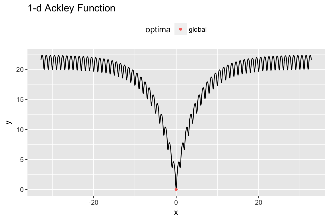
The best way to illustrate the process of algorithm design in ecr is by example. Assume we aim to find the global minimum of the highly multimodal one-dimensional Ackley-Function. The function is available in the R package smoof and may be initialized as follows:

library(ecr)
#> Lade nötiges Paket: BBmisc
#> Lade nötiges Paket: smoof
#> Lade nötiges Paket: ParamHelpers
#> Lade nötiges Paket: checkmate
library(ggplot2)
library(smoof)
fn = makeAckleyFunction(1L)
pl = autoplot(fn, show.optimum=TRUE, length.out = 1000)
print(pl)

One-dimensional Ackley test function.

Writing the evolutionary loop by hand

We decide to use an evolutionary \((30 + 5)\)-strategy, i.e., an algorithm that keeps a population of size mu = 30, in each generation creates lambda = 5 offspring by variation and selects the best mu out of mu + lambda individuals to survive. First, we define some variables.

MU = 30L; LAMBDA = 5L; MAX.ITER = 200L
lower = getLowerBoxConstraints(fn)
upper = getUpperBoxConstraints(fn)

In order to implement this algorithm the first step is to define a control object, which stores information on the objective function and a set of evolutionary operators.

control = initECRControl(fn)
control = registerECROperator(control, "mutate", mutGauss, sdev = 2, lower = lower, upper = upper)
control = registerECROperator(control, "selectForSurvival", selGreedy)

Here, we decide to perform mutation only. The best mu individuals (regarding fitness values) are going to be selected to build up the next generation.

Finally, the evolutionary loop is implemented.

population = genReal(MU, getNumberOfParameters(fn), lower, upper)
fitness = evaluateFitness(control, population)
for (i in seq_len(MAX.ITER)) {
    # sample lambda individuals at random
    idx = sample(1:MU, LAMBDA)
    # generate offspring by mutation and evaluate their fitness
    offspring = mutate(control, population[idx], p.mut = 1)
    fitness.o = evaluateFitness(control, offspring)

    # now select the best out of the union of population and offspring
    sel = replaceMuPlusLambda(control, population, offspring, fitness, fitness.o)
    population = sel$population
    fitness = sel$fitness
}
print(min(fitness))
#> [1] 0.04438188
print(population[[which.min(fitness)]])
#>            x 
#> -0.009814595

Black-box approach

Since the optimization of a continuous numeric function is a standard task in EC, ecr ships with a black-box function ecr(...) which basically is a customizable wrapper around the loop above. A lot of tasks can be accomplished by utlizing this single entry point. However, often EA design requires small tweaks, changes and adaptations which are simply impossible to realize with a black box regardless of their flexebility.

The optimization of our 1D Ackley-function via ecr(...) might look like this:

res = ecr(fitness.fun = fn, representation = "float",
  n.dim = getNumberOfParameters(fn), survival.strategy = "plus",
  lower = lower, upper = upper,
  mu = MU, lambda = LAMBDA,
  mutator = setup(mutGauss, sdev = 2, lower = lower, upper = upper),
  terminators = list(stopOnIters(MAX.ITER)))
print(res$best.y)
#> [1] 0.0004027943
print(res$best.x)
#> [[1]]
#>            x 
#> 0.0001005639 
#> attr(,"fitness")
#> [1] 0.0004027943